Web Page: http://geog.ucsb.edu/~kclarke
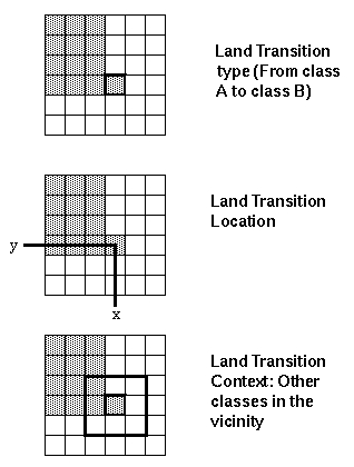
Our latest work has extended the scope of the modeling component of the work to land transitions. Land cover transitions are the product of three underlying properties (Figure 1). First, the transition represents a discrete change of state. This means that if a location, such as a point, polygon, or pixel, at one time is in state A and and some other time in state B, then we can say that a state change has taken place. In some cases, land use and land cover transitions are rather more subjective in their classification than this statement implies. For example, a wooded forest lot may become the back yard of a luxury residence, and so change from forest to residential, changing use without changing cover. Nevertheless, we will assume that type transitions are discrete and definitive for the arguments in this work.
Secondly, land transitions have spatial location. For every transition between states, there is a geographic location that can be ascribed to that place. This information is not recorded when information is retained only about class changes, yet is important if land transition models are to simulate transitions, especially dynamically. In general, we can state that the places are not spatially independent. There is a strong degree of spatial autocorrelation between land transitions, some positive, and some negative. For example, in a rural area a small cross-roads may become the location for a cluster of residences. A single pixel may change from forest to urban. In the next step, land immediately adjacent to the buildings may be cleared of trees for gardens and farming. Thus the two transitions are directly spatially adjacent because they share a common origin in a sequence of events. At the broader scale, city edges are characterized by spatially autocorrelated transitions, as are resorts, farming at the periphery, and so forth.
Thirdly, land transitions are contextually linked. A simplistic model
of land transitions, for example, could compute a transition matrix, select
a state at random, draw a random number that matches a transition, select
at random a pixel in the old state, and enforce change on that pixel. This
ignores, however, the fact that the pixel selected for change has a spatial
context, or a local "state neighborhood." Thus a pixel surrounded by eight
adjacent pixels of the same state might be considered far less likely to
change than a pixel surrounded by pixels all in different states.
Figure 1: The three types of land transitions.
These three transition factors, what might be called state transition, location, and spatial context, should form the basis of a majority of transitions in a model of land transition, but obviously not all. Occasionally, particular transitions happen at random. Forest becomes wasteland because of a wildfire, or a pleasant spot in the forest is selected as the location for a residence. The transitions these changes initiate within the immediate vicinity are not random. The forest to wasteland example is unlikely to change to urban use without water, power or roads access, but may now be suitable for agricultural use as pasture. Thus once change has begun, however initated, a set sequence may be followed that is non random, both in further transitions on tha same location, and in adjacent transitions.
In addition, the motive force behind land transitions is usually associated with a single land cover type. In an ecological model of species, for example, an endangered or an invading species may be making all the spatial rules. In the broad land cover context, the dominant driving transition is the one converting unsettled land to human settlement, the urbanization land transformation. Prior work has used this approach to model urbanization from the past into the future. It is also possible to model a more full set of land use/cover transitions with similar methods, given that ultimately all land transitions are the result of the ongoing urbanization process itself.
Models of land transitions start by examining the state transition. A factor of interest here is that although for any two images at times 0 and 1 a state transition probability matrix T cab be computed, without further data it is impossible to state whether or not these transitions are stable. While it can fairly safely be assumed that the rows of transition probabilities sum to one, any given probability may actually vary randomly, systematically, or chaotically. Raising the matrix to a large power to produce a "static equilibrium state" therefore, is speculative to the highest degree. We propose that the probabilities are stable for short periods, but should be recomputed as many times as there are data available to do so.
The T matrix can be generated by having at least two identical land cover maps at different time periods. For example, for the two symthetic images in figures 2 and 3, the matrix in figure 4 was generated.
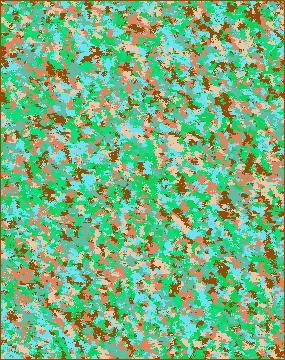
Figure 2: Synthetic Land Use at Time 0.

Figure 3: Synthetic Land Use at Time 1.
Figure 4: Land Cover Transition Matrix for figures 2 and 3. Counts and Probabilities
14786 [0.9936]    14 [0.0009]    23 [0.0015]    13 [0.0009]    17 [0.0011]    12 [0.0008]    16 [0.0011]
 12   [0.0008] 14160 [0.9937]    14 [0.0010]    19 [0.0013]    12 [0.0008]    14 [0.0010]    19 [0.0013]
 16   [0.0012]     5 [0.0004] 13696 [0.9943]    17 [0.0012]    11 [0.0008]    12 [0.0009]    18 [0.0013]
 16   [0.0011]    13 [0.0009]    16 [0.0011] 14297 [0.9934]    17 [0.0012]    16 [0.0011]    17 [0.0012]
 13   [0.0009]    14 [0.0010]     9 [0.0006]     9 [0.0006] 14016 [0.9954]     9 [0.0006]    11 [0.0008]
  7   [0.0005]    11 [0.0008]    10 [0.0007]     7 [0.0005]    17 [0.0012] 14413 [0.9945]    27 [0.0019]
 19   [0.0012]    18 [0.0012]    20 [0.0013]    14 [0.0009]    18 [0.0012]    18 [0.0012] 15336 [0.9931]
With only two land use/cover maps, obviously nothing can be determined about the statistical nature of the probabiltities. With three maps, a crude model of change or at least a variance estimate can be made.
The driving force of urbanization can be added by using an external model for these transformations, here we will use the Cellular Automaton Model, to generate a set N of newly grown pixels in a cellular landscape. The number of newly urbanized pixels is used as the driver for probabilities derived from the land transition matrix. For example, having normalized the probabilities in L to produce T, then with x urban transition pixels, x = X/N calls can be made to the random number generator. The result is that further land transitions (excluding those related to urban) are generated within a single model iteration.
The deltatron is an artificial "agent" of change that has "life" in change space. Whenever a land cover transition takes place, a cell is "born." A deltatron attempts to change the land use/cover class of the immediate neighborhood. A deltatron will survive one iteration if in the next time step another transition of the same "to" type (i.e. same column in the transition matrix) happens in the eight-cell neighborhood of the transition. In this next step, no further transition can happen to the original pixel. Some deltarons are "killed" at random. Others die because no further change takes place in the vicinity. Thus eventually, even changed pixels can change at some time in the future.
The impact of the deltatrons is to act as cellular automata. Periods of growth and decline in change take place naturally. There are phase transitions in change, and the system seems to fluctuate between spatial structure (with fairly simple diffusion of growth outward from an initial point) and chaos. During periods of rapid driver impact (urban growth), obviously more deltatrons are created and they have more impact and interaction, resulting in a more spatio-temporally chaotic pattern. In periods of low growth, simple diffusion is normally follwed by death and the land use/cover change is "absorbed" by the landscape.
Figure 4 (left) shows an animation of thirty Deltatron cycles for the synthetic land use data. The land cover maps undergoing the transitions are on the right. As is often the case in the real world, it is hard to determine that land cover changes are taking place at all from the spatial image. It was this fact that encouraged us to work in "delta" space to begin with.
In addition, we will be "scaling up" the entire model to cover the entire coterminous 48 United States at about 4km resolution. Sources of historical growth will be Atlases, USGS maps, the National Atlas, and other sources including the DMSP. Sources of land use in digital form will be the GIRAS files and the more contemporary land characterization images from the EROS Data Center. It is hoped to both assess the feasibility of scaling the model, and to make a set of projections for use in global change research.