1. BUFFERING

2. POINT IN POLYGON

3. POLYGON OVERLAY

4. SPATIAL INTERPOLATION

5. DENSITY ESTIMATION

Transformations create new objects and data sets from existing objects and data sets

buffering takes points, lines, or areas and creates areas

every location within the resulting area is either:

in/on the original object

within the defined buffer width of the original object

example

discrete object:

for every object, result is a new polygon object

new objects may overlap

field (objects cannot overlap):

every location on the map has one of two values:

inside buffer distance
outside buffer distance

find all households within 1 mile of a proposed new freeway

and send them notification of proposal

find all areas of Los Padres National Forest beyond 1 mile from a road

find all liquor stores within 1 mile of a school

and notify them of a proposed change in the law

find households within a fixed service radius

CSISS cookbook and UCI's medical center

raster and vector versions

vary the object's buffer width according to an attribute value

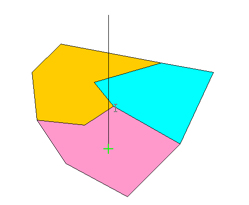
e.g. noise buffers depending on road traffic volume

vary the rate of spread according to a friction field

only in raster
e.g. travel speed varies

Thiessen polygons for point objects

the area closest to each point forms a polygon

Determine whether a given point lies inside or outside a given polygon

assign a set of points to a set of polygons

e.g. count numbers of accidents in counties
e.g. whose property does this phone pole lie in?

draw a line from the point to infinity

count intersections with the polygon boundary

inside if the count is odd
outside if the count is even

diagram

point must lie in exactly one polygon

point can lie in any number of polygons, including zero

algorithm for a coverage

what if the point lies on the boundary?

special cases

Create polygons by overlaying existing polygons

how many polygons are created when two polygons are overlaid?

example

find overlaps between two polygons

e.g. a property and an easement

creates a collection of polygons

overlay two complete coverages

creates a new coverage

e.g. find all areas that are owned by the Forest Service and classified as wetland

in vector or raster

in raster the values in each cell are combined, e.g. added

areal interpolation

source zones with known data
target zones with unknown data
estimates based on areas of overlap
spatially extensive or spatially intensive

California counties and three-digit ZIPs

major computing workload

indexing

swamped by slivers

tolerance

What is interpolation?

intelligent guesswork

an interval/ratio variable conceived as a field

temperature
soil pH
population density

sampled at observation points

needed:

values at other points
a complete surface

a contour map
a TIN
a raster of point values

inverse-distance weighting (IDW)

Kriging (geostatistics)

estimates are averages of the values at n known points

known values z₁,z₂,...,z_n

unknown value z = Sum over i (w_iz_i) / Sum over i (w_i)

where w is some function of distance, such as:

w = 1/d^k

w = e^-kd

an almost infinite variety of algorithms may be used, variations include:

the nature of the distance function
varying the number of points used
the direction from which they are selected

is the most widely used method

objections to this method arise from the fact that the range of interpolated values is limited by the range of the data

no interpolated value will be outside the observed range of z values

peaks and pits will be missed if they are not sampled

outside the area sampled the surface must flatten to the average value

other problems include:

how many points should be included in the averaging?

what to do about irregularly spaced points?

how to deal with edge effects?

summary: IDW is popular, easy, but full of problems

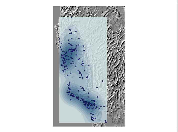
ozone concentrations at CA measurement stations

objectives:

1. estimate a complete field, make a map
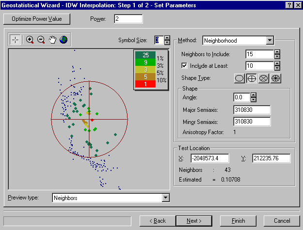
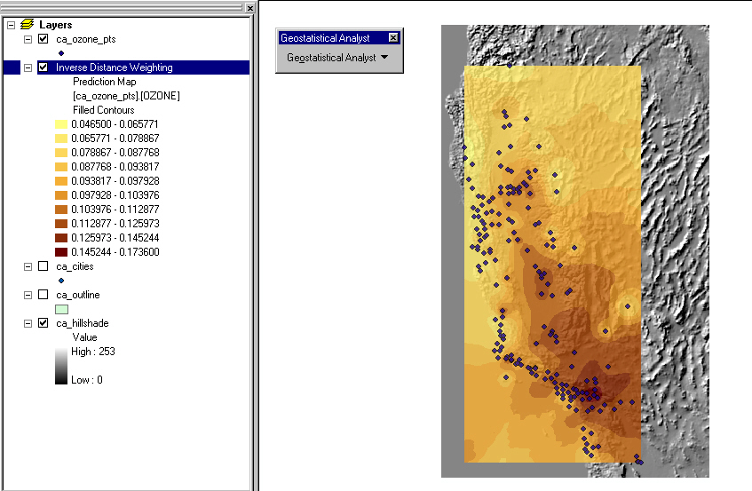
2. estimate ozone concentrations at other locations

e.g. cities

data sets:

measuring stations and concentrations (point shapefile)
CA outline (polygon shapefile)
DEM (raster)
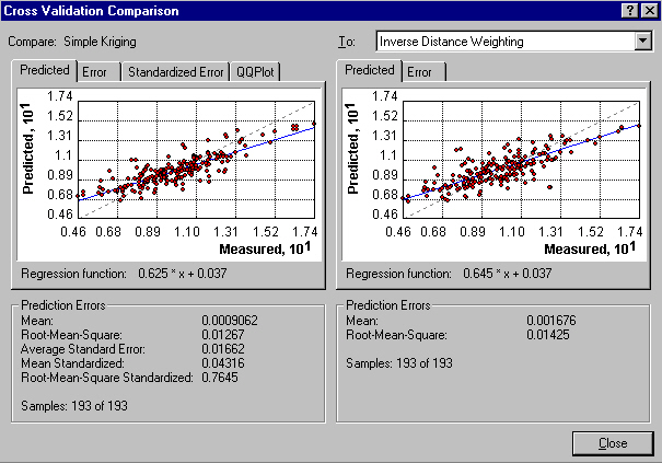
CA cities (point shapefile)

IDW wizard in Geostatistical Analyst

opening screen defines data source

next screen defines interpolation method

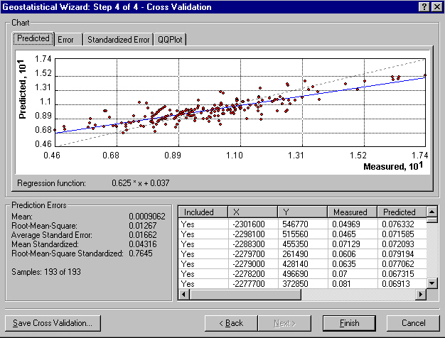
which power of distance? (2)
how many sectors? (4)
how many neighbors in each sector? (10-15)

next screen gives results of cross-validation

results map

things to notice

amount of detail where there is no data

generally smooth surface

highs in LA, S central valley

developed by Georges Matheron, as the "theory of regionalized variables", and D.G. Krige as an optimal method of interpolation for use in the mining industry

the basis of this technique is the rate at which the variance between points changes over space

this is expressed in the variogram which shows how the average difference between values at points changes with distance between points

Kriging is based on an analysis of the data, then an application of the results of this analysis to interpolation

vertical axis is E(z_i - z_j)², i.e. "expectation" of the difference

i.e. the average difference in elevation of any two points distance d apart

d (horizontal axis) is distance between i and j

most variograms show behavior like the diagram

the upper limit (asymptote) is called the sill

the distance at which this limit is reached is called the range

the intersection with the y axis is called the nugget

a non-zero nugget indicates that repeated measurements at the same point yield different values

in developing the variogram it is necessary to make some assumptions about the nature of the observed variation on the surface:

simple Kriging assumes that the surface has a constant mean, no underlying trend and that all variation is statistical

universal Kriging assumes that there is a deterministic trend in the surface that underlies the statistical variation

in either case, once trends have been accounted for (or assumed not to exist), all other variation is assumed to be a function of distance

the input data for Kriging is usually an irregularly spaced sample of points

to compute a variogram we need to determine how variance increases with distance

begin by dividing the range of distance into a set of discrete intervals, e.g. 10 intervals between distance 0 and the maximum distance in the study area

for every pair of points, compute distance and the squared difference in z values

assign each pair to one of the distance ranges, and accumulate total variance in each range

after every pair has been used (or a sample of pairs in a large dataset) compute the average variance in each distance range

plot this value at the midpoint distance of each range

fit one of a standard set of curve shapes to the points

"model" the variogram

once the variogram has been developed, it is used to estimate distance weights for interpolation

interpolated values are the sum of the weighted values of some number of known points where weights depend on the distance between the interpolated and known points

weights are selected so that the estimates are:

unbiased (if used repeatedly, Kriging would give the correct result on average)

minimum variance (variation between repeated estimates is minimum)

problems with this method:

when the number of data points is large this technique is computationally very intensive

the estimation of the variogram is not simple, no one technique is best

since there are several crucial assumptions that must be made about the statistical nature of the variation, results from this technique can never be absolute

simple Kriging routines are available in the Surface II package (Kansas Geological Survey) and Surfer (Golden Software), in the GEOEAS package for the PC developed by the US Environmental Protection Agency, and in ArcInfo 8 as an add-on Geostatistical Analyst

example

selection of method

simple Kriging

ordinary Kriging allows for a trend
co-Kriging includes a correlated variable
indicator Kriging is for binary data

analysis of the variogram

fitting a model
directional effects

how many neighbors?

cross-validation

things to notice

similar pattern

less detail in remote areas
smoother

rebounds to the mean at the edge

better cross-validation

Suppose you had a map of discrete objects and wanted to calculate their density

density of population

density of cases of a disease

density of roads in an area

density would form a field

density estimation is one way of creating a field from a set of discrete objects

count the number of points in every cell of a raster

measure the length of lines, e.g. roads

result depends on cell size

result is very noisy, erratic

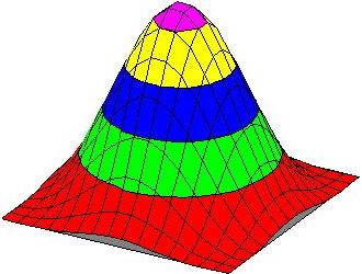
think of each point being replaced by a pile of sand of constant shape

add the piles to create a surface

example kernel

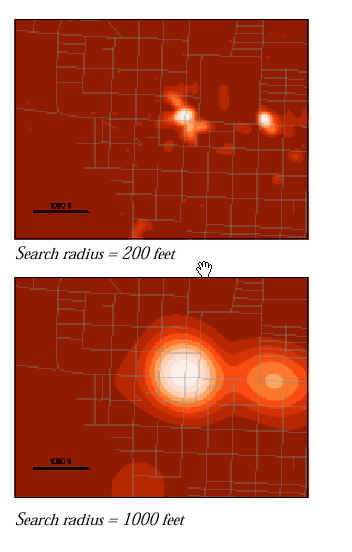
width of the kernel determines the smoothness of the surface

density of ozone measuring stations

using Spatial Analyst

kernel is too small (radius of 16 km)

kernel radius 150 km

what's the difference?