LECTURE 3: COVERAGES

1. FLAT-FILE GIS

Canada Geographic Information System

magnetic tape storage

reduce a map to a linear sequence of bits

all maps classified land

soil capability

forest capability

recreation capability

current land use

...

maps scanned as rasters

vectorized for compression, calculation of area, apparent accuracy

the arc as the basic record

strung end to end on tape

left poly ID, right poly ID, number of points, x,y,x,y,x,y,x,y,...

all input and output involved tape

2. THE RELATIONAL MODEL

Database management systems

pre-1970s

programs handled input and output

commands to read, write hard disk, diskettes, tapes

a GIS had to do its own

many lines of code

the database approach

all reading and writing through a simple interface

no need for user to care about details of disk, tape etc

easy to replace database layer

with another vendor's product

database handles basic housekeeping

knows the details of format

knows about variables

e.g. house price

knows units of measurement

knows range (negatives not possible)

can export data to another system easily

"export" command

enables simple operations

total a column of numbers

search for records satisfying some condition

the relational model

emerged in the 1980s as the dominant model

replaced the hierarchical and network models

Oracle, Access, Informix, Empress, ...

needs to be widely applicable, so can't assume too much

must assume something, or it wouldn't be useful

the rows define the cases, objects, instances, records of some class of objects

the columns define the known properties or attributes

all of the objects in the class must have the same kinds of properties

in GIS, must be all points, all lines, all areas, all pixels, etc.

5 attendees (rows)

4 attributes (columns)

What can go in the columns?

data (integers, floats, dates, text)

BLOBs (images, music, video)

hyperlinks to web sites

links to initiate programs

e.g. links to GIS

compare Excel

passengers with reservation details

aircraft with maintenance, schedule details

crew with schedule, pay details

a model of an enterprise

county data (polygons)

customer data (points)

road data (lines)

flight number in a passenger record

flight number in a crew record

flight number in an aircraft record

passenger table relates McCain to a flight

aircraft record relates flight to an aircraft

user doesn't need to know these are in separate tables

A GIS example:

table of car accidents

county as an attribute

table of counties

link any accident to attributes of the county it occurred in

county as the common key

relation

a table

tuple

a record in a table

a row in a table

key

a subset of attributes that is

unique for each record

no redundancy

can't throw away any attribute in the key

e.g. phone directory

phone number is unique key

last name, first name, street address is unique

drop any part and the result is not necessarily unique

still possible to be non-unique?

join

merger of two tables

using key to add attributes from Table 2 to records of Table 1

not symmetrical

number of records in join is determined by Table 1

reversible

normalization

spatial join

use location as the common key

match point to point, point to polygon, polygon to polygon

very flexible

no need to worry about implementation

user can ask questions that involve more than one table

linkage of tables is automatic

The relational model applied to GIS

the georelational model

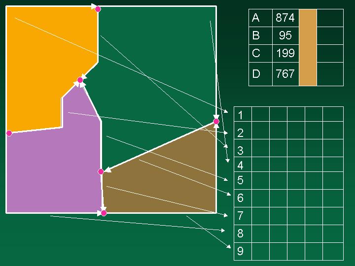
representing maps in the relational model

ARC/INFO circa 1980

polygons

arcs

nodes

 Coverage slide 2

 Coverage slide 3

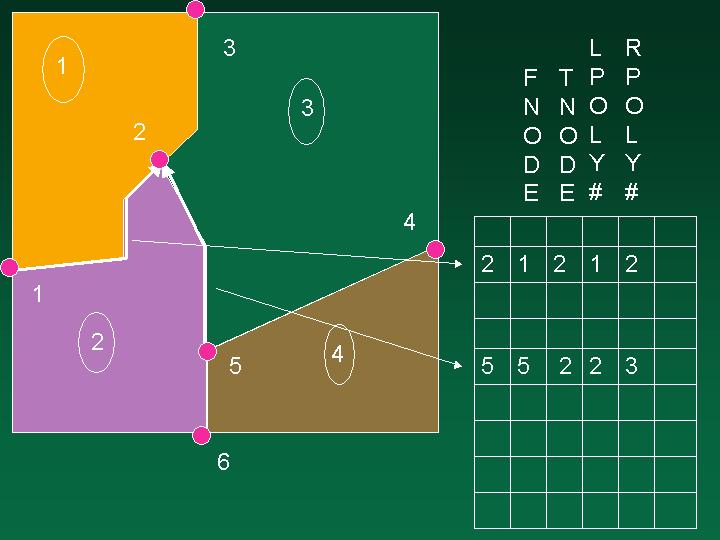
Using arcs as the basic unit

avoids double representation of internal boundaries

easier to build the database

easier to edit and maintain

keeps track of 'topology'

which nodes are connected by which arcs

which polygons are separated by which arcs

a concept strongly associated with the coverage model

coverages have more topology than shapefiles

1) relationships between objects

every arc points to two polygons

the "outside world" is a special polygon

every arc ends at two nodes

nodes have any number of arcs

but sometimes limited to three

polygons have any number of arcs

but sometimes limited by design

Euler's Theorem

P-A+N=2

or 1 if the outside world is not counted

2) integrity of objects

polygons must be closed

building topology

assembling lines into arcs and polygons

forming junctions

removing overshoots

Polygon attribute table (PAT)

Arc attribute table (AAT)

Tics (TIC)

Annotation (LAB)

Tolerances (TOL)

INFO relational database

Microsoft Access

shapes (points) stored in special file (ARC)

not directly viewable

all points within one polygon have the same attributes

all points must lie in exactly one polygon

a field

values at each point are classes

a categorical coverage

an area class map

resource management

forest stands

soil type

vegetation cover class

land use class

the cadaster

land ownership parcels

demographics

census data

data by state

data by county

marketing data by market area

population by ZIP

the choropleth map

the area class map

coverages capture the field view of the world

a continuous world

one value of a variable at every point

sharp changes in value as boundaries are crossed

points

lines

arcs

TINs

grids