LECTURE 11: ANALYSIS OF SURFACES
1. TYPES OF DIGITAL TERRAIN MODELS
1. TYPES OF DIGITAL TERRAIN MODELS
Digital terrain models are very commonly used in GIS
three types of data
three data models
also LiDAR point clouds
raster
regularly spaced spot heights
DEM (digital elevation model)
USGS 30m data
1 arc second for the lower 48
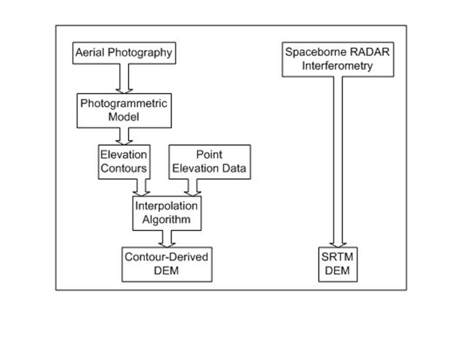
derived from topographic maps
contour-to-grid interpolation
Mission Creek
global GTOPO30
1km data
derived from multiple sources
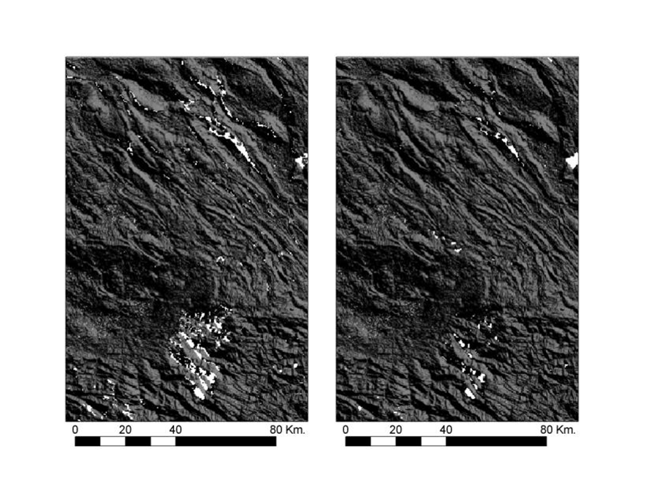
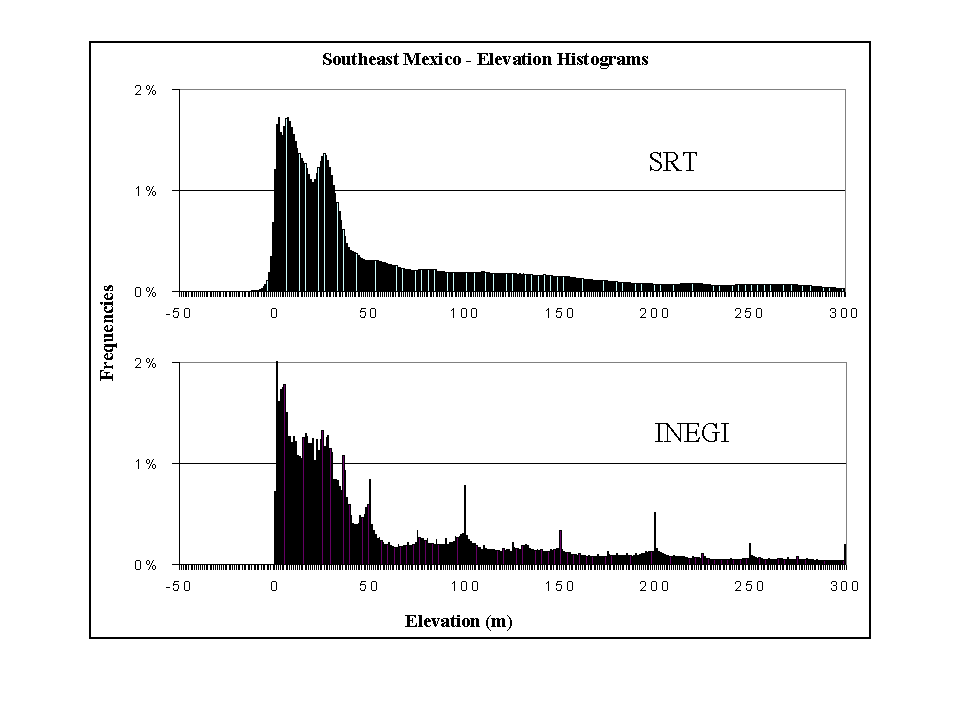
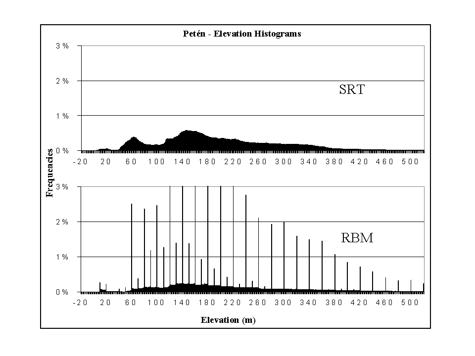
Shuttle Radar Topography Mission (SRTM)
3 arc second
interferometric radar
54S to 60N
holes
water
sand dunes
associated artifacts
from contours
CTOG
from stereoplotter profiling
fjords
from "soft" photogrammetry
digitized contours
Digital Line Graph (DLG) data
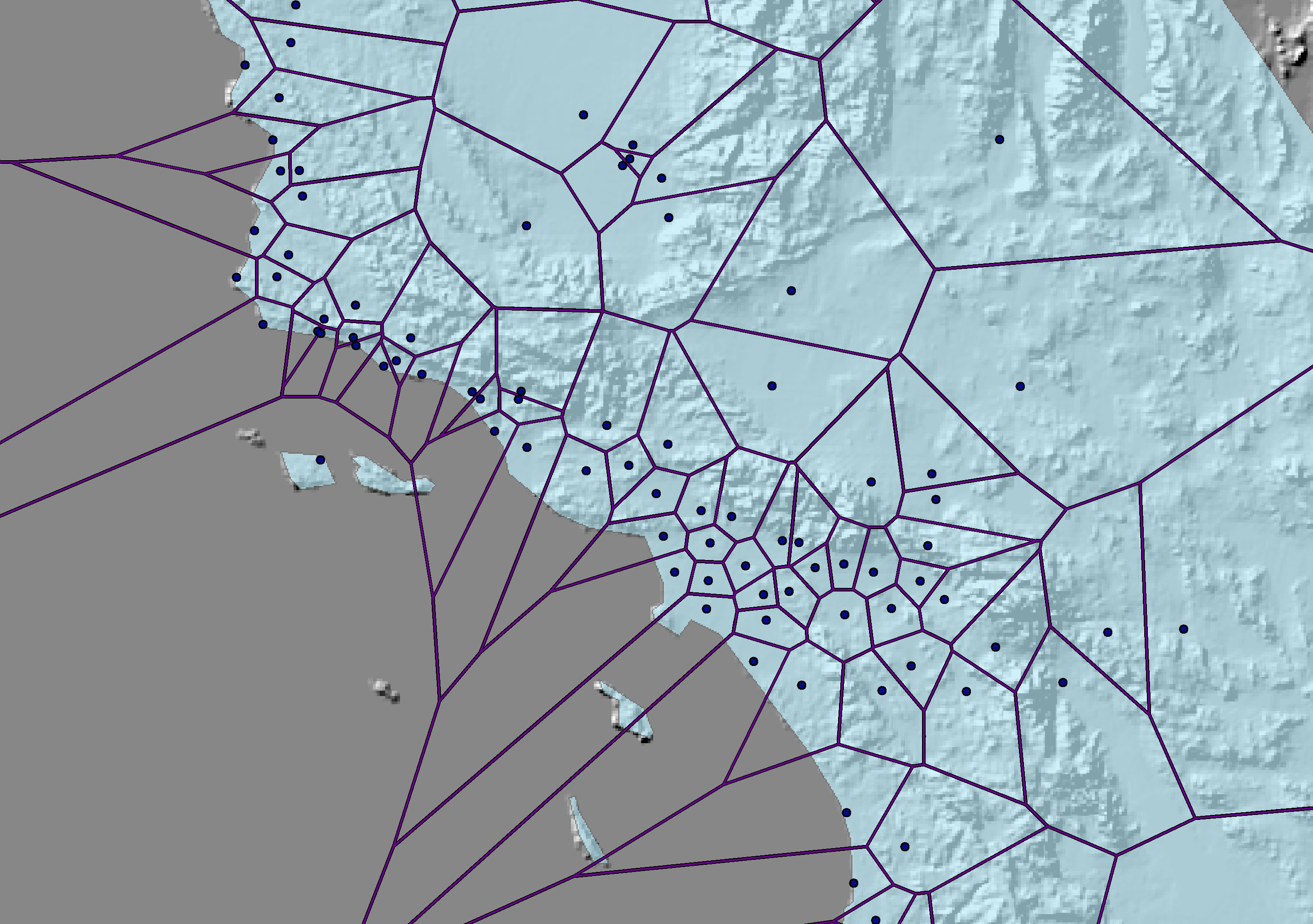
triangulated irregular network (TIN)
a mesh of triangles
Delaunay triangles
constant slope within each triangle
breaks of slope at edges
many applications
triangles used in contouring
accuracy issues
positioning of vertices
best approach?
terrain type
glaciated
mass wasting
canyons
Google Earth example
can estimate many other properties from them
slope
aspect
solar insolation
best routes
viewsheds
drainage patterns
best logging techniques
best ski runs
risk of landslide, avalanche
DEM provides best data model for most of these
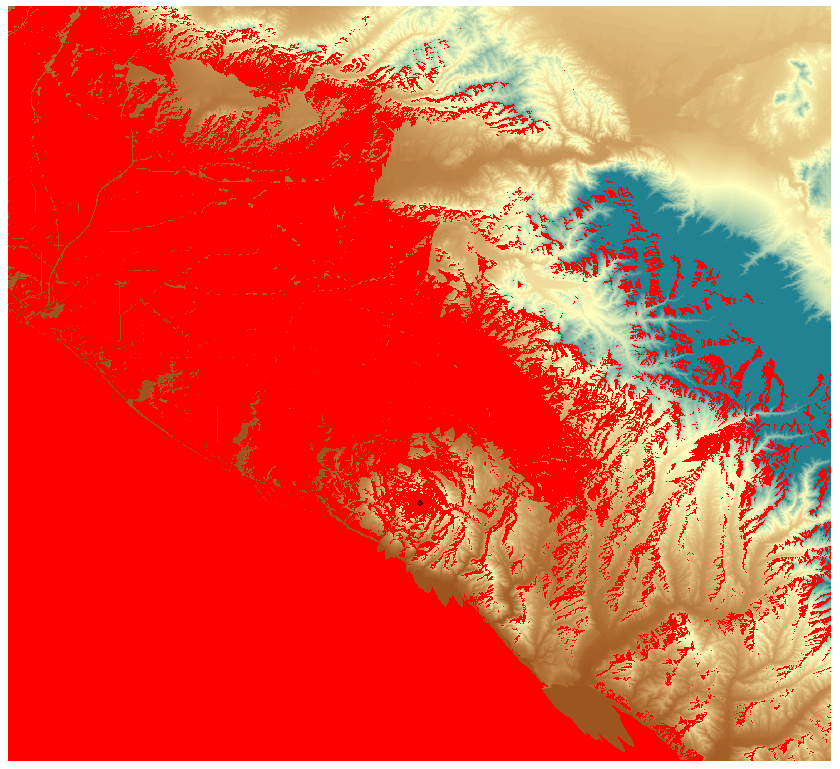
slope
estimated by fitting a plane to a 3x3 neighborhood centered on each point
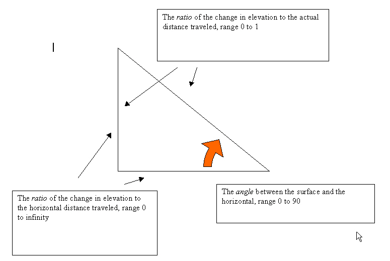
how is slope defined?
angle (0-90)
percentage
rise over run
horizontal run or run on the slope?
ArcGIS uses the tangent
a "slope map" often creates polygons from ranges of slope
classify, convert to features
losing information
aspect
the direction of steepest slope
cyclic variable problem
e.g. calculating mean aspect
determining drainage networks, watersheds
compare cell's elevation to the elevation of its neighbors
flow is to the lowest neighbor
if no neighbors are lower, cell is a pit
how many possible directions?
4 = "rook's case"
8 = "queen's case"
example DEM
| 10 | 9 | 11 | 12 |
| 8 | 7 | 6 | 7 |
| 5 | 4 | 3 | 4 |
| 5 | 0 | 1 | 5 |
flow directions (4 moves)
| 3 | 3 | 3 | 3 |
| 3 | 3 | 3 | 3 |
| 2 | 3 | 3 | 4 |
| 2 | 0 | 4 | 4 |
flow directions (8 moves)
| 4 | 4 | 5 | 6 |
| 4 | 4 | 5 | 6 |
| 4 | 5 | 6 | 6 |
| 3 | 0 | 7 | 7 |
determining the watershed
an attribute of each point on the network
identifies the region upstream of that point
begin at the specified cell
label all cells which drain to it
then all which drain to those, etc.
until the upstream limits of the basin are defined
the watershed is the polygon formed by the labeled cells
determining the network
connect the moves with arrows
a zero on the edge of the array is a channel which flows off the area
too many channels
density determined by cell size not real world
may want to accumulate water as it flows downstream
channels begin only when a threshold volume is reached
accumulation of volume
start by setting each cell to zero
beginning at each cell, add one to it and all cells downstream of it
flow directions (8 moves)
| 4 | 4 | 5 | 6 |
| 4 | 4 | 5 | 6 |
| 4 | 5 | 6 | 6 |
| 3 | 0 | 7 | 7 |
accumulated flow
| 1 | 1 | 1 | 1 |
| 1 | 2 | 4 | 1 |
| 1 | 2 | 8 | 1 |
| 1 | 16 | 3 | 1 |
ArcGIS coding scheme
E = 1
SE = 2
S = 4
SW = 8
W = 16
NW = 32
N = 64
NE = 128
other values indicate ties
how do networks obtained from DEMs differ from real ones?
areas of uniform slope generate too many parallel streams
need to randomize
streams flow mostly to the lowest neighbor
but sometimes to second-lowest neighbor
Orange County DEM
calculate slope
measure ease of travel
combine slope and elevation
define an origin point
find best paths from this point to all others
zonal analysis of elevation by tract
spatial join
predicting drainage
comparison to reality