(Notation_1)
4th International Conference on Integrating GIS and Environmental
Modeling(GIS/EM4):
Problems, Prospects and Research Needs. Banff, Alberta, Canada, September2 -
8, 2000.
A coupled cellular automaton model for land use/land cover dynamics
GIS/EM4
Jeannette Candau
Steen Rasmussen
Keith C. Clarke
Abstract
The Clarke Urban Growth Model (UGM), a cellular automaton (CA) that simulates urban growth through time, is coupled with the Deltatron Land Use/Land Cover Model (DLM), which extends representation capabilities to multiple land cover class transitions, to create a new, more robust model, SLEUTH. The DLM depicts urban expansion into the landscape produced by the UGM. The DLM uses CA-based rules, class-transition probabilities, and local topography to create deltatrons (bringers of change) and enforce land class transitions within homogenous land class areas, as well as at the interface of land use/land cover types. These deltatrons enforce spatial and temporal auto-correlation in the land cover transition process. The dynamics of the land cover change are defined through a four-step process: (i) Initial Change, (ii) Cluster Change, (iii) Propagate Change, and (iv) Age Deltatrons. For the first time, these simulated urban and land cover processes, previously only formulated as computer algorithms, have been translated into a functional form with their corresponding pseudo code, which both clarifies their character and makes it easier to compare with other approaches. In addition, this formalization makes it simpler to include other important simulated human-made and natural processes in future coupled modeling.
SLEUTH was tested using synthetic data sets and then applied at 1-km resolution to the Mid-Atlantic Integrated Assessment (MAIA) area of the Environmental Protection Agency. After the model went through extensive calibration for the MAIA area, forecasts of urban growth and other land cover change were simulated through 50 Monte Carlo iterations starting in 1992 to produce a probability-related growth map of land cover classes for the year 2050. A corresponding map was produced that describes the uncertainty related to any cell's predicted land-cover class. Together, these maps provide a valuable tool to describe predicted land cover change and its uncertainty. By bringing the maps back into a geographic information system, spatial context can be given to land class forecasts and the associated level of confidence assessed. Additional land cover dynamics could easily be added to the current approach. This approach is the first of its kind, and is applicable to any geographical region. Cellular automata as complex systems models are valuable tools for forecasting how the spread of urbanization could shape future land cover patterns, at many spatial scales.
Keywords
Dynamic modeling, urban modeling, land cover modeling, land use modeling,
urban development impacts, cellular automata, visualization of uncertainty, complex system modeling,
urban dynamics, land cover dynamics.
Complex System Modeling with Cellular Automata
Evolving from previous work, a model of land cover change has been developed and applied to a regional dataset. The cellular automaton Clarke Urban Growth Model (UGM) simulated the effect of topography, adjacency, and transportation networks on the patterns of urbanization though time (Clarke, Gaydos, and Hoppen 1996). This model was calibrated using historical data for a region compiled in a geographic information system (GIS) (Clarke, Hoppen, and Gaydos 1996). The results were then used to forecast the development of the regional urban system into the future (Clarke and Gaydos 1998). The land cover change deltatron model explored in this paper, is tightly coupled with the UGM, and also utilizes historical, digital data maps to calibrate model performance. The models together are referred to as SLEUTH by reference to the models’ input data requirements: Slope, Land cover, Exclusion, Urban, Transportation, Hillshade. The sum being greater that its parts, SLEUTH, using only the clues given by known data input, seeks to discover emergent form in a dynamic landscape.
The evolution of land cover patterns is a process governed by a large number of forces both natural to the environment and imposed by human disruption. The state of the system at any given time is the result of the interplay of its many components. Trying to identify the intricate inter-relationships of these many drivers has often led to frustration. Recently, complex systems approaches suggest the multitude of interactions that take place on a largescale, or individual level, forms the basis of system wide, or aggregate, behavior.
The foundation for this complex system approach was pioneered by Von Neuman (1966) who presented the idea that a type of computing machine could not only reproduce itself, but could generate a machine of greater complexity than the original. This concept was expressed in the form of a cellular automata (CA). The best known simple example of a CA is the Game of Life developed by John Conway (Gardener, 1970). The game is executed upon a regular tessellation of cells, in this case a grid of uniform, square pixels. The cells may exist in one of two states: alive or dead. It was discovered that, depending upon the configuration of the initial conditions, complex spatial patterns could emerge though repeatedly applying the behavior rules to the grid. In recent years CA has been applied in various fields, and many examples can be found regarding the subject of urban modeling and form (White and Engelen 1993; Papini and Rabino1997; Batty and Xie 1994; Clarke, Hoppen and Gaydos 1996).
We have extended the scope of our research from modeling urban development to include how this expansion in turn affects sequential land transitions (Clarke 1997, Candau 2000). Physical patterns of land cover change may be shown three ways. The first is the tendency of one land class to expand into another where the two meet. This is the most common type and may be seen as the expression of a land cover type “growing” into its neighbors as topography and neighborhood resistance allows. The second is a less predictable occurrence of a new land cover type being introduced into an otherwise homogenous area. Both of these trends, though they begin at a discrete point and time, may signal similar transition events in their neighborhood. This third occurrence, a perpetuation of change, enables transition forces to be carried across a landscape. The deltatron model seeks to build upon these concepts of how, where and when land cover dynamics take place.
Definition of Urban Dynamics
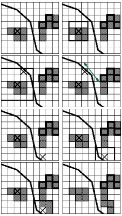
The urban growth dynamic implemented in UGM is defined through four steps that we call (i) Spontaneous Growth, (ii) New Spreading Centers, (iii) Edge Growth, and (iv) Road-Influenced Growth. In this section we first discuss the different growth steps and the functional form of their dynamics, and then depict an example of the growth step followed by the pseudo code that defines this step.
Two measures of suitability affect the likelihood of urbanization throughout the growth process. The suitability is defined by an exclusion layer (for example, water, swamps, etc.) and by slope. Slope above 21% cannot be urbanized. Given that the local slope (slope (i,j)) is below 22%, the slope_coefficient determines the weight of the probability that the location (i,j) may be built upon.
(i) Spontaneous Growth
Spontaneous growth (figure 1) defines the occurrence of random urbanization of land. In the cellular automaton framework this means that any non-urbanized cell on the lattice has a certain (small) probability of becoming urbanized in any time step. Thus, whether a given cell U(i,j,t) at coordinate (i,j) at time t will be urbanized at time t+1 can be expressed by
|
(Notation_1)
|
where the parameter dispersion_coefficient ( diffusion_coefficient in previous literature (Clarke, Hoppen, Gaydos 1996)) determines the (small) spontaneous, global urbanization probability, and the slope_coefficient parameter determines the weighted probability of the local slope. The stochasticity of the process is indicated by random. If the cell is already urbanized or excluded from urbanization, it will not change, and therefore the ability to transition also depends on the cell’s own current value.
|
|
Spontaneous Growth:
F(dispersion_coefficient, slope_coefficient) { } end spontaneous growth |
| Figure 1 Spontaneous growth example and pseudo code. | |
(ii) New Spreading Center Growth
The next urban growth step is defined though the dynamics of new spreading centers (figure 2). As the name indicates, this step determines whether any of the new, spontaneously urbanized cells will become new urban spreading centers. The global parameter, breed_coefficient, defines the probability for each new urbanized cell U(i,j,t+1) to become a new spreading center U'(i,j,t+1), given two neighboring cells also are available for urbanization
|
(Notation_2)
|
where (k,l) are nearest neighbors to (i,j). If the cell is allowed to become a spreading center, two additional cells adjacent to the new spreading center cell also have to be urbanized. Thus an urban spreading center is defined as a location with three or more adjacent urbanized cells. The actualization of this step is dependent upon the slope_coefficient-weighted topography and the availability of neighborhood cells to make the transition.
 |
New Spreading Center Growth: |
| Figure 2 New spreading center growth example and pseudo code. | |
(iii) Edge Growth
Edge-growth dynamics (figure 3) define the part of the growth that stems from existing spreading centers. This growth propagates both the new centers generated in step ii in this time step, time (t+1), and the more established centers from earlier times. Thus, if a non-urban cell has at least three urbanized neighboring cells, it has a certain global probability to also become urbanized defined by the spread_coefficient, given it is possible to build on the cell (slope_coefficient). Thus this edge growth can be expressed by
|
(Notation_3)
|
where (k,l) belongs to the nearest neighborhood of (i,j).
 |
Edge Growth: |
| Figure 3 Edge growth example and pseudo code. | |
(iv) Road-Influenced Growth
The final growth step, road-influenced growth (figure 4), is determined by the existing transportation infrastructure as well as the most recent urbanization done under steps ii and iii. With a probability defined by breed_coefficient, newly urbanized cells (at time t+1) are selected, and the existence of a road is sought in their neighborhoods. If a road is found within a given maximal radius (determined by road_gravity_coefficient) of the selected cell, a temporary urban cell is placed at the point on the road that is closest to the selected cell. Next, this temporary urban cell conducts a random walk along the road (or roads connected to the original road) where the number of steps is determined by the parameter dispersion_coefficient. The final location of this temporary urbanized cell is then considered as a new urban spreading nucleus. If a neighboring cell to the temporary urbanized cell (on the road) is available for urbanization, it will happen (randomly picked among possible candidates). If two adjacent cells to this newly urbanized cell are also available for urbanization it will happen (randomly picked among candidates). Thus the creation of the temporary urbanized cell on the road is defined by
|
(Notation_4.1)
|
where i,j,k,l,m, and n are cell coordinates, and R(m,n) defines a road cell. The random walk on the road may be expressed by
|
(Notation_4.2)
|
where (i,j) are road cells neighboring (k,l). If we define the location of the temporary urbanized cell at the end of the random walk by (p,q), the new adjacent urban spreading center will be defined by
|
(Notation_4.3)
|
and two additional adjacent urbanized cells may be added using
|
(Notation_4.4)
|
where (i,j) and (k,l) belong to the nearest neighborhood of (p,q). Note how this step is similar to notation 3.
 |
Road-Influenced Growth: |
| Figure 4 Road-influenced growth example and pseudo code. | |
Deltatron Dynamics
The urbanization process drives the changes in the non-urbanized land cover. The dynamics of the land cover change are defined through a four-step process: (i) Initial Change, (ii) Cluster Change, (iii) Propagate Change, and (iv) Age Deltatrons. In the following section we first explain the different growth steps and the functional form of their dynamics, and then depict an example of the step followed by the actual pseudo code that defines this step.
Initial Conditions
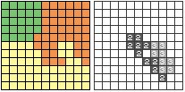
In the following, the land cover change dynamics are assumed to have been active for at least three update cycles so that besides the land cover space (lattice), a corresponding "aged deltatron space or layer" also exists (figure 5). Deltatrons, which are “bringers of change", track the spatial and temporal effects of land transitions. They do not contain land class values, but act as a reference of where and when a change has occurred. Depending upon the age of the deltatron, its locally associated land class may be available for propagating change, or holding it in its current state. We use L(i,j,t) to define the land cover class (value) at (i,j) at time t and D(i,j,t) as the corresponding age in the deltatron layer. Note that the current deltatron age (value of D(i,j,t)) is different from the current time t in the simulation.
 |
Input data configuration for Deltatron Dynamics example: |
| Figure 5 Initial conditions of deltatron example. | |
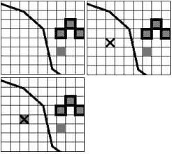
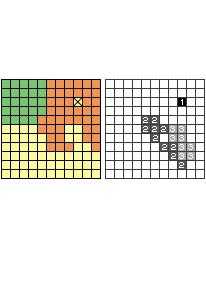
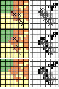
(i) Initiate Change
Each newly urbanized cell (newly_urbanized) is now assumed to induce a potential change in land cover (figure 6) and, as a result, produce a deltatron in a randomly selected non-urbanized cell
| (Notation 5) |
where the selected cell either will stay the same or transition to another land cover type. This is determined by a probability weighted by the average slopes (average_slopes) for each land cover class, the historical land cover changes, and the slope of the current cell. These probabilities are defined such that more frequent land use changes, as well as historically occurring correlations between slopes and land uses, are weighted appropriately. They define a local Markov chain (a Random Markov Field) with transition probabilities between the current land cover class and all other land use classes (vector of transition probabilities by multi_state_markov_chain). If a transition occurs, a new deltatron is created. Only cells that are not already deltatrons can be recruited as a location for a new deltatron.
 |
Initiate Change: G(number of new pixels) { } } } end initiate change |
| Figure 6 Initiate change example and pseudo code. | |
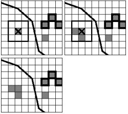
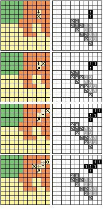
(ii) Create Change Cluster
The Create Cluster dynamics (figure 7) are defined as an aggregation process (growth) of these newly created deltatrons and the associated land cover transition. The parameter cluster_size, controls how large each new deltatron cluster can grow
|
(Notation_6)
|
where L(k,l) are neighboring cells to the new deltatron cell at location (p,q). Each new cell that is picked (at random among the possible neighboring cells) is now changed to the same land cover class as the new deltatron, or remains unchanged, defined by the weighted slope and historic transition probabilities (local two_state_markov_chain, also defines a Random Markov Field). Note that in this step, the cells can only change to the land use class the associated deltatron has, or remain unchanged. In step i the cell can potentially change to any one of the land cover classes weighted by the appropriate probabilities.
 |
Create Change Cluster: { } } end Create Change Cluster |
| Figure 7 Create change cluster example and pseudo code. | |
The newly transitioned cell now acts as the land cover change, aggregation center. Again a random cell from its neighborhood is tested for land cover change with the same probabilities (to remain unchanged or change to the same new land cover class). To encourage clustering, a certain probability exists that the aggregation center will be moved back to the original (first) deltatron location (i_center, j_center) as the process continues, until terminated by the size of the parameter cluster_size.
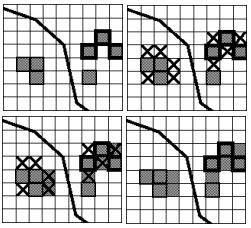
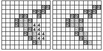
(iii) Propagate Change
The Propagate Change dynamics (figure 8) is very similar to the Edge Growth step in the Urban Growth dynamics. All non-deltatron cells which are neighbors to at least two deltatron cells with an age of two (they were created in time t-1) are tested against the same weighted probability to either remain unchanged or change to the same land cover type as a neighboring deltatron’s land cover type
|
(Notation_7)
|
 |
Propagate Change: |
| Figure 8 Propagate change example and pseudo code. | |
(iv) Age Deltatrons
Finally, in the Age Deltatrons step (figure 9) all deltatrons are aged to the next time step. The number or cycles a deltatron may live is defined by min_years_between_transitions. If they become “older” then this maximum deltatron age, they “die” and can, in principle, be recruited as a new potential deltatron in the next growth cycle
|
(Notation_8)
|
 |
Age Deltatrons: { } end age deltatrons |
| Figure 9 Aging deltatrons example and pseudo code. | |
Testing the Coupled CA Model: The MAIA Case Study
The Mid-Atlantic Integrated Assessment (MAIA) study area is
a region designated by the Environmental Protection Agency for the implementation
of research, monitoring, and assessment of ecological conditions (http://www.epa.gov/maia/html/about.html).
It includes seven states and the District of Columbia on the eastern coast of
the United States: Delaware,
District of Columbia, Maryland, North Carolina, New York, Pennsylvania, Virginia,
West Virginia.
The U. S. Geological Survey (USGS), in cooperation with the University of California, Santa Barbara, applied SLEUTH to the MAIA region at a data resolution of 1-km. Using a temporal GIS database, an extensive calibration of the model (Clarke, Hoppen and Gaydos 1996) for the area was performed. To create the temporal database urban data were generated from U.S. Census Bureau data for the years 1950, 1970, 1980, and 1990. USGS 1:2,000,000 Digital Line Graphs of interstate and major highways formed the base transportation map for the year 1980. Maps from American Automobile Association were used as ancillary data to identify the extent of interstate highways in 1950 and 1970. Two Anderson Level I classified land cover maps from the years 1975 and 1992 were used to define the land cover class-transition matrix. For calibration, the earliest land cover map provided initial conditions for the deltatron model. The most recent land cover map was used to measure how well the spatial patterns of land cover evolution were modeled for that year. In the final model year, a map of simulated land cover was produced and compared on a per pixel basis with the known data. This new comparison metric was added to the calibration process so that the deltatron model might influence adjustment of the coefficients.
Probabilistic Forecasting
Once model calibration for the MAIA region was complete, urban growth and land cover change was simulated into the future. Beginning in the data year 1992 (figure 10), the model was run for 50 Monte Carlo iterations to the year 2050. From this process, two prediction maps were produced that describe the likelihood and character of land cover change. The first (figure 11) is a map of the most probable forecasted land class for the year 2050. Each location is classified by its “winning” land cover type. That is, by the land class present most often over the 50 Monte Carlo iterations. Figure 12 shows the pixels that changed class from 1992 to 2050. They are color classified by the class they changed to. The urban growth around already established urban areas is clear.
 |
 |
| Figure 10 MAIA 1992 land cover. | Figure 11 MAIA 2050 forecasted land cover. |
|
|
|
 |
 |
| Figure 12 MAIA 2050 land cover, color classified by forecasted land type. | Figure 13 MAIA 2050 contrast-stretched cumulative uncertainty map. |
A second image produced by SLEUTH is a map (figure 13) of uncertainty that is associated with the land cover forecasts. It is calculated by counting the number of times each class was at a given location over all Monte Carlo iterations. If a location is found to always have the same land cover when the year 2050 is reached, its uncertainty value is zero and will appear black in the image. However, if one land class is equally likely as another of being present, there is a high degree of uncertainty related to modeled class transition. The higher a pixel’s value in the uncertainty map the lighter it will appear, and the less confidant we are in the model’s prediction at that location. In the case of pixels that are classified as “NODATA”, nothing is known about their state, and their associated uncertainty is also at a maximum.
Conclusions and Discussion
Cellular automata as complex systems models are valuable tools for forecasting how the spread of urbanization could shape future land cover patterns at different spatial scales. The basic SLEUTH dynamics of urbanization, and resulting land cover change, have successfully been tested on eight mid-Atlantic entities showing the strength and the potential value of a coupling between urban growth and land cover changes. This approach is the first of its kind and is applicable to any geographical region. Its current form is quite general, but allows for higher levels of complexity. For example, additional natural land cover dynamics easily could be added to the current approach through ecological succession (for example, grass land to woodland). Further, these simulated processes, previously only formulated as computer algorithms, have been translated into a functional form with their corresponding pseudo code, which both clarifies their character and makes it easier to compare with other approaches. In addition, this formalization makes it simpler to include other important simulated human-made and natural processes in future coupled modeling (Heiken et. al. 2000).
The cumulative land cover and uncertainty maps show new information about the spatial and temporal relations of land transitions. Together, these maps provide a valuable tool to describe predicted land cover change and its uncertainty. By bringing the maps back into a GIS, spatial context can be given to land class forecasts and the associated level of confidence assessed.
SLEUTH is written in the C programming language and implemented on a variety of platforms, including a CRAY supercomputer in parallel mode, on SGI and SUN workstations, and on PC systems running LINUX. The model’s portability has allowed it to be applied to various urban regions around the world, and at various scales. Additional application sites include the Rio Grande Basin, New Mexico; Santa Barbara, Calif; and Lisbon, Portugal. Areas of study that will be modeled within the next year include Mexico City, Mexico; Philadelphia, Penn; and the Santa Clara Valley, Calif. Complete documentation, including publications, implementation instructions, links to study site data, and downloadable source code may be found on-line at the Project Gigalopolis web site (http//:www.ncgia.ucsb.edu/projects/gig/).
References used
Batty M, Xie Y. 1994. From cells to cities. Environment and Planning B 21:31-48.
Candau JT. 2000. Probabilistic land cover transition modeling using deltatrons. Proceedings of the 37th Annual URISA Conference; 2000 Aug 19-23; Orlando, FL.
Clarke KC, Gaydos L, Hoppen S. 1996. A self-modifying cellular automaton model of historical urbanization in the San Francisco Bay area. Environment and Planning B 24: 247-261.
Clarke KC, Hoppen S, Gaydos L. 1996. Methods and techniques for rigorous calibration of a cellular automaton model of urban growth. Third International Conference/Workshop on Integrating GIS and Environmental Modeling; 1996 Jan 21-25; Santa Fe, New Mexico.
Clarke KC. 1997. Land transition modeling with deltatrons. <http://www.ncgia.ucsb.edu/conf/landuse97/>. Accessed 2000 Jul 17.
Clarke KC, Gaydos L. 1998. Loose coupling a cellular automaton model and GIS: long-term growth prediction for San Francisco and Washington/Baltimore. International Journal of Geographical Information Science 12 (7): 699-714.
Gardener M. 1970. The fantastic combinations of John Conway's Game of Life. Scientific American 23: 120-23.
Heiken G, Valentine G, Brown M, Rasmussen S, George D, Green R, Jones E, Olesen K, Andersson C. 2000. Modeling cities: the Los Alamos Urban Security Initiative. Public Works Management & Policy 4 (3): 198-212.
Papini L, Rabino G. 1997. Urban cellular automata: an evolutionalry prototype. In: Bandini S, and Mauri G. [editors]. ACRI ’96. Proceedings of the second conference on cellular automata for research and industry; (pp. 1996 Oct 16-18; Milan, Italy. Berlin: Springer. p 147-157.
Von Neumann J. 1966. Theory of Self-Producing Automata. Urbana and Chicago: University of Illinois Press.
White R, Engelen G. 1993. Cellular automata and fractal urban form: a cellular modeling approach to the evolution of urban landuse patterns. Environment and Planning A 25: 1175-1199.
Authors
Jeannette Candau, Physical Scientist, U. S. Geological Survey
Graduate Student, Department of Geography
University of California, Santa Barbara, 3611 Ellison Hall, Santa Barbara, CA
93106.
Email:jcandau@usgs.gov, Tel: +1-805-893-5178, Fax: +1-805-893-5178.
Steen Rasmussen, Staff Scientist,
Geoanalysis and CNLS,
Los Alamos National Laboratory, Los Alamos, NM, 87545
and Santa Fe Institute, 1399 Hyde Park Road, Santa Fe, NM 87501.
Email: steen@lanl.gov, Tel: +1-505-665-0052, Fax: +1-505-665-6459.
Keith C. Clarke, Professor of Geography
University of California, Santa Barbara, 3611 Ellison Hall, Santa Barbara, CA
93106.
Email: kclarke@geog.ucsb.edu, Tel: +1-805-893-9674, Fax: +1-805-893-3146